A very useful technique for suspension tuning is to use histograms and wheel sway speed analysis to evaluate spring and damping settings. In particular, these graphs relate the wheel speed (positive speed values indicate compression, negative values indicate extension) and the percentage of samples (statistically the time elapsed by each shock absorber in the compression and extension phases). In a theoretically ideal suspension configuration, we will have a symmetrical histogram with a bell curve like the one shown in the figure below which, in particular, is characterized by:
- Low speed compression: 25%
- Low speed rebound: 25%
- High Speed Compression: 25%
- High speed rebound: 25%
Remember: the hight speed bump and the hight speed rebound of shock absorber spring occur to step over bumps, potholes and curbs of the circuit. The low speed bump and the low speed rebound of the spring occur during braking (front wheels in compression and rear in extension) or in acceleration (front wheels in extension and rear in compression) or when cornering, while the car tilts (the inner wheels go in rebound and the outer wheels in compression).

Note: in the histogram below (MoTeC telemetry) the low compression and rebound speed zones are represented in dark blue while the analogous high speed zones in lighter blue.
In the aggressive ACC setup prepared for the Brands Hatch circuit, on the other hand, we have a more rigid slow rebound (low speed rebound) and softer slow compression (low speed bump) at the front; this graphically results in an asymmetrical bell that extends slightly to the right (i.e. towards the bump), as shown in the figure below, since the softer low bump (soft) lets the suspension move more in compression than in extension (keep in mind that this weak asymmetry does not indicate any problem).
This is not particularly significant, but if you want a symmetrical bell, you have to reduce the stiffness of slow extension or increase the stiffness of slow compression until symmetry is achieved. Small asymmetries are not a problem; instead, if the peak of the curve is for example on the border between low speed compression and hight speed compression (or on the border between low speed rebound and hight speed rebound), this is an indication that something is not working as it should. In fact, highly asymmetrical graphs indicate that the damper is setup badly in bump or rebound, fast or slow.
The image below shows the histogram relating to the rear suspension. From the graph we can see that the curve is extremely flat with even a slight dip in the center of the low speed zone. This indicates that the rear shocks are too soft and need to be stiffened.

If we compare the aggressive setup with a softer setup (figure below) we will notice in this second case, a general flattening of the bells due to a generalized increase in the oscillation speed of the shock absorber pistons, even at the extremes of the graph (high speed areas).

Especially at the front, the peak of the curve must be quite pronounced. Skaven Zverov (in revision 1.6 of his guide) and Nils Naujoks, Director of the Red Bull Racing Esports Team, suggest that at the 0.0 mm/s point that divides the compression zone from the extension zone, the peak should be around at 12%, exactly as shown in the ideal graph.
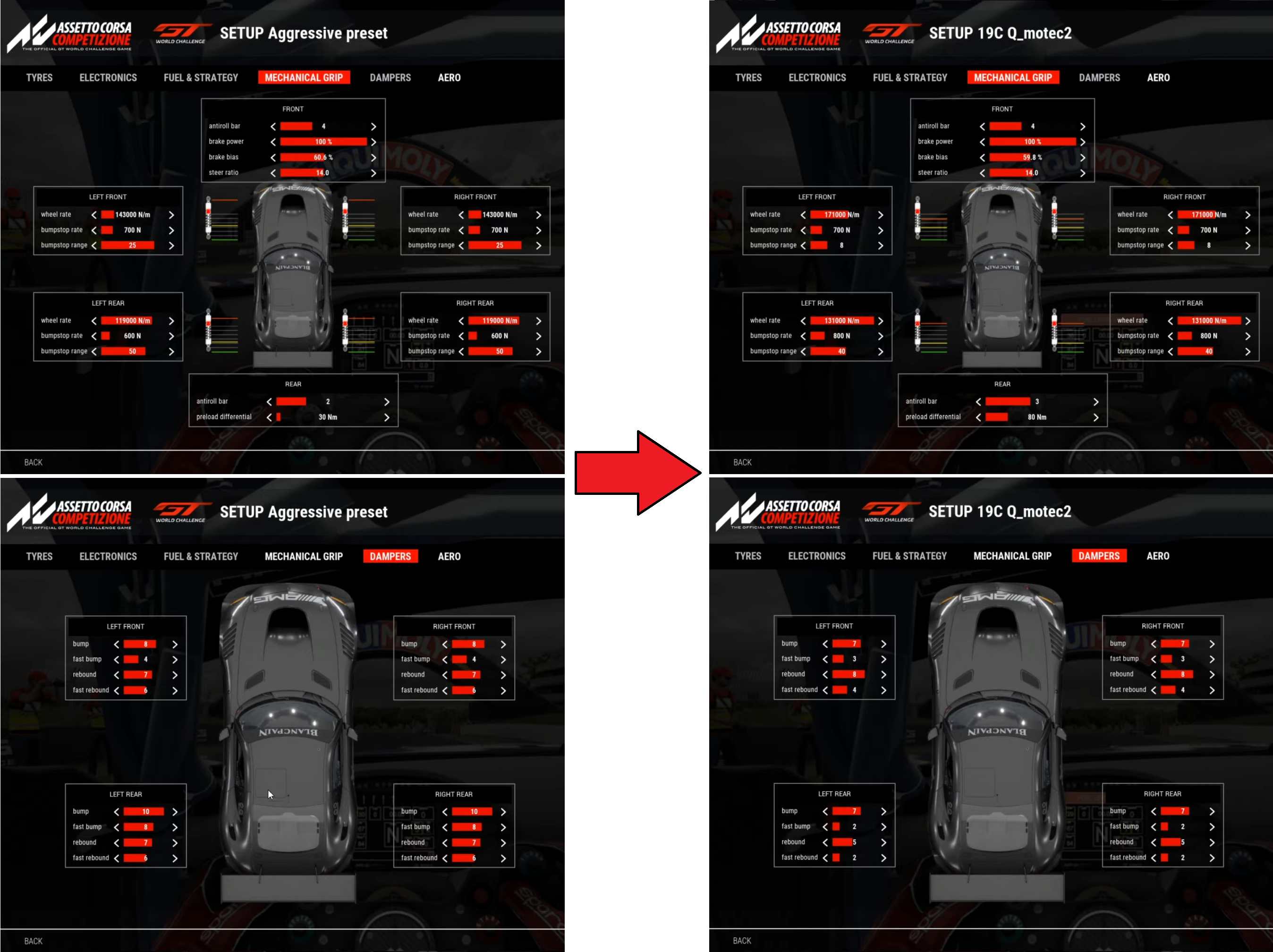
In the figure below we can see the comparison between the aggressive setup (mechanical grip and dampers sections) of the Mercedes AMG GT3 (left), relative to the Mount Panorama circuit, with the version of the same setup suitably modified by Nils Naujoks (right) for obtain a histogram with a more pronounced peak, comparable with the bell curve of the ideal graph (to enlarge the image click here).

It can easily be seen that, with regard to the mechanical grip, the stiffness of the springs both at the front and at the rear has been increased, although in the latter case the margin for modification was much less. Less significant and useful changes for the specific purpose have been made to the stiffness of the bumpstop rate and to the excursion of the suspension (bumpstop range). These changes were in fact made eminently to reduce the car’s pitch under braking and acceleration. Overall, these interventions were sufficient to bring the peak of the histogram from 8% to about 12%, as shown in the figure below.

The changes to the dampers setup were instead necessary to obtain a perfectly symmetrical bell. In consideration of the fact that at the front the bell extended slightly to the left (i.e. towards the extension), the rebound was stiffened by a click at the front (in fact, if in the histogram the rebound bar is too high, first you have to increase rebound damping) and then it was also necessary to soften the bump by a click. We omit to illustrate the modifications to the rear dampers, as the procedure for obtaining a symmetrical histogram also at the rear is the same as that previously described for the front.
But how do we know if the setup changes are working? Or if the car’s behavior has significantly improved?
We can in fact make corrections to the setup if the histogram is highly asymmetrical or if the bell is flat or barely pronounced but we cannot actually know if this will result in a gain in chronometric terms (or at least it is not possible to read it from the histogram of the shock absorbers).
So let’s go to the “suspension travel” worksheet and analyze the telemetry relating to turn 4, one of the most problematic of the Brands Hatch circuit.

In the following figure, lower graph, we can see the oscillations of the right rear wheel which is on the outside in curve 4. This wheel is subject to greater shocks related to the disconnections on this side of the track, when exiting the corners (the white line is the one relating to the soft setup and the blue line is related to the very rigid setup).

Note: starting from ACC patch 1.3, the resolution with which MoTeC exports data has gone from 20 Hz to 200 Hz frequency and, therefore, it is no longer necessary to filter the traces of the various channels.
We enlarge the graph in correspondence with curve 4 (image below) and we see that the rigid setup (blue line) would seem to absorb shocks although it oscillates in an extremely contained manner; compared to zero, the suspension moves in extension up to 28 mm and in compression up to 47 mm. If we take into consideration the softer setup (white line), we see that the suspension has a wider excursion (ranging from 14 mm in rebound to 50 mm in compression, again with respect to the zero of the graph).

Zooming in on the area in red again, the difference in suspension oscillation between the stiff and soft setup is much more evident. In particular, we note that the rigid setup (blue line) has a smaller amplitude and period of oscillation than the soft setup (white line). This last characteristic also determines an evident phase difference.

Ultimately, the two configurations have a completely different behavior towards holes, bumps and depressions present on the track.
Let’s now analyze the “wheel speed” worksheet. We can see that in correspondence of the bumpy, the rolling speed of the rear wheels (magenta for the left rear and blue for the right rear) is greater in the rigid setup than the speed of the corresponding wheels with the soft setup. This happens because the suspension is so stiff that it does not adequately absorb shocks and the wheel jumps until it almost loses contact with the track, resulting in skidding. The spin of the wheels at this particular point of the circuit occurs for just over 1/10 of a second. This translates into a loss in terms of lap time, although it is not excluded that the rigid setup can make us gain in other points of the track.

Finally, let’s see how this lack of absorption of disconnections translates into the behavior of the steering wheel, analyzing the “driver” worksheet.

In this sheet we can see that with the soft setup (white line), at the exit of curve 4, there are no corrections with the steering wheel which is kept rotated by about 100° until the exit of the curve and then almost perfectly realigned (0° of steering wheel angle) in a straight line, unless an irrelevant slight correction. With regard to the rigid setup (red line), it can be seen that at the exit of curve 4 there is a lower steering wheel angle (rotation equal to about 50°) but at a certain point there is a realignment and then two large corrections before the definitive straightening of the steering wheel at the straight. These two corrections are symptoms of oversteer that force the driver to counter-steer.
Remember: if the work on the steering wheel lasts less than 2/10 of a second, this steering movement is called “driver feedback” and can be ignored during the telemetry analysis; it is an unnecessary movement but which makes the driver safer and has no practical effect on the behavior of the car. But if the work on the steering wheel lasts more than 2/10 of a second (even in our case the work on the steering wheel lasts half a second), this phenomenon is called the “handling issue”; this deprives the driver of confidence with the car and involves a considerable loss in terms of lap time.
Finally, the essential function of the shock absorbers is summarized in the figure below.

Note: for the preparation of this guide, reference was made to the following video tutorials:
